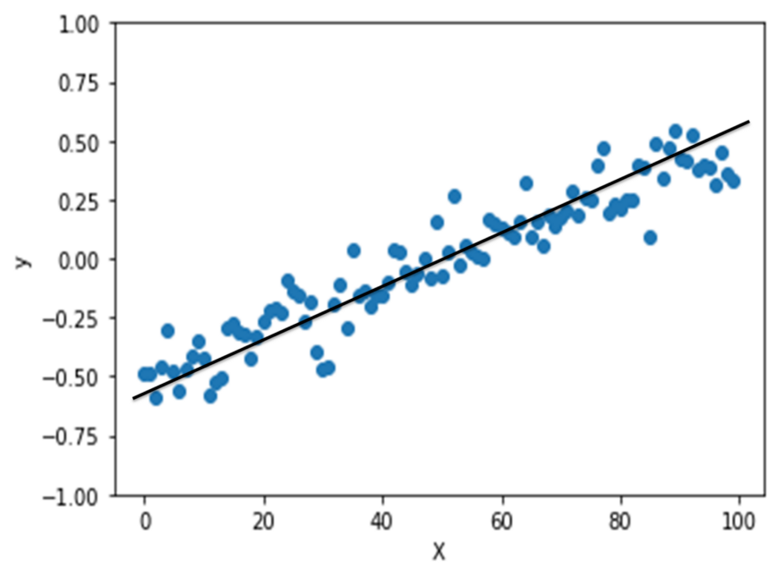
My journey into linear regression has just began and as I understand the most basic thing about linear regression is about fitting a line to a data. Well as it sounds it is simple and equally at the same time challenging too. The deal is to have the concept clarity.


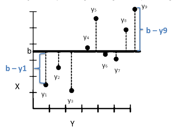
Assuming we are working on a data-set and we have this data and it has been plotted on a X Y graph.
We are likely to add a line to the data so that we can see the trend and check what the best line that can represent the trend is. The horizontal line that cuts through the average value is the line which is the least likely to be desired for and is probably the worst fit of all. But like it is said there is no better way to start than the zero ground, the horizontal line gives a good starting point for an analysis on how to find the optimal line to fit the data.
We can now draw a line from this point up to the line that cuts across the average Y value for this data-set. The distance between the line and the first data point equals ‘b’- Y1, the distance between the line and the first data point equals ‘b’-Y2, and so on it will continue as b’-Y3…. till ‘b’-Y9.
We need to square the values :
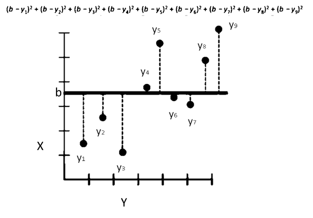
If you note Y4 is greater than ‘b’ since it’s above the horizontal line and hence b’ -Y4 the value will be negative and that will be no good as it will start subtracting from the total and make the fit appear better than it really is the fifth data-set is even higher relative to the horizontal line this distance is going to be very negative.
Taking absolute value made math very tricky so the best solution that came up was squaring each term. Squaring ensures each term is positive. The equation below shows the distance the data points have from the horizontal line.
Applying the above will give us the measure of how well the line will fit the data. As we understand residuals are the differences between the real data and the line, the Sum of squared residuals is the value that we get summing the square of these values.
We have to see how good the fit is if by rotating the line till the time we meet the sweet spot in between the horizontal and the vertical residual lines. If we notice we can see that the sum of squared residuals goes down when we start rotating the line , but that it’s possible to rotate the line too far in the sum of squared residual starts going back up again.
The Generic line equation:
The generic line equation is: y = a * x + b
Where ‘a’ is the slope of the line and ‘b’ is the y intercept of the line (that’s the location on the Y axis that the line crosses when X equals zero).
We want to find the optimal values for A and B so that we minimize the sum of squared residuals.
In more general math terms the sum of squared residuals is this complicated mathematical equation (a * x1 + b) –y1)² + (a * x2 + b) –y2)² + ……
Let me make it simpler the first part (a * x1 + b) is the value of the line at X1 and the second part y2 is the observed value at X1. So what we are really doing in this part of the equation is calculating the distance between the line and the observed line
Since we want the line that will give us the smallest sum of squares this method for finding the best values for A and B is called Least squares.
If we plotted the sum of square residuals versus each rotation we get something like below
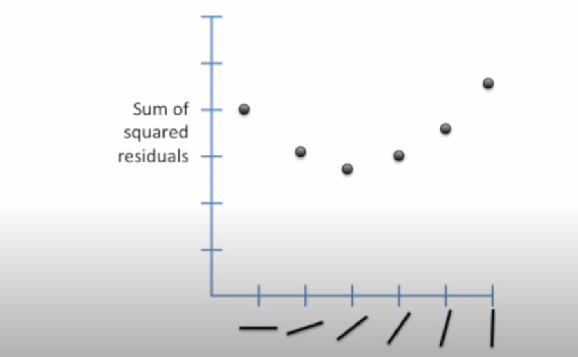
Where on the Y axis we have the sum of squared residuals and on X axis we have got each different rotation of the line.
Finding the optimal rotation for the line?
The answer is we take the derivative of this function, the derivative tells us the slope of the function at every point.
The slope at the point on the far left side is pretty steep. As we move right the steepness reduces to the best point where we have the least squares is zero an then it moves back again.
We need to remember that different rotations are just different values for A the slope and B the intercept.
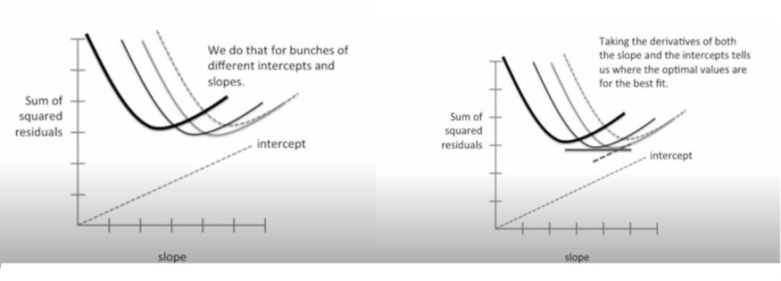
Different values for the slope and intercept results in different sum of squares. We do that for a bunch of different intercepts and slopes. Taking the derivatives of both the slope and the intercepts tells us where the optimal values are the best fit.
Few concepts to understand:
- We want to minimize the square of the distance between the observed values and the line
- We do this by taking the derivative and finding where it is equal to zero
- The final line minimizes the sum of squares (it gives the “least squares”) between it and the real data Y = ax+b

